Umbrella sampling with Replica Exchange

Umbrella Sampling with Replica Exchange

Objective and Overview

The objective of this tutorial is to learn how to use the MMTSB Tool Set in combination with CHARMM to carry out replica exchange umbrella sampling simulations.

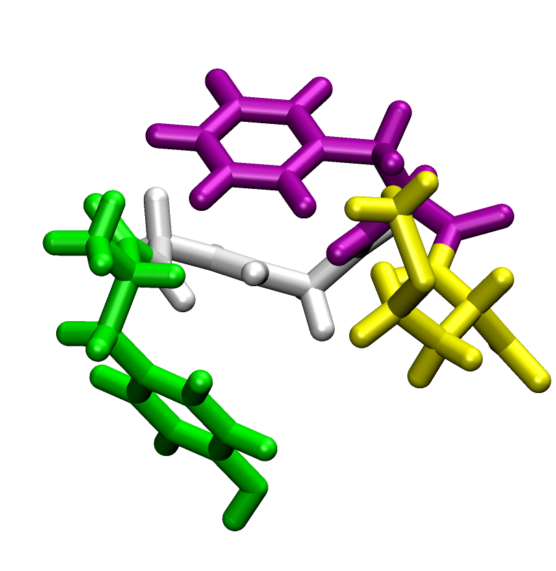
In this tutorial we will study met-enkephalin, a small peptide with the sequence YGGFM. The goal is to describe the conformational sampling in aqueous solvent at 300K. One structure of the peptide is shown on the right.

1. Initial setup

We will begin with the structure from the PDB file metenk.pdb. Minimize the structure with the following command:

    
  minCHARMM.pl -par gb,blocked metenk.pdb > metenk.min.pdb

We will use implicit solvent (the GBMV model will be used) and blocked terminal to avoid charge-charge interactions of between the termini that are by default zwitterionic. No further equilibration is needed.

2. 1D Umbrella replica exchange run

Met-enkephalin is known to sample both compact and extended states at 300K. A good reaction coordinate to describe the difference between compact and open states is the end-to-end distance between the C-alpha positions of the terminal residues (1 and 5). Here we will carry out umbrella sampling along this reaction coordinate in order to obtain the free energy as a function of the end-to-end distance.

We will use replica exchange sampling to enhance sampling over standard umbrella sampling. In this case, each replica will apply a different biasing function (at a different end-to-end distance value). In contrast to temperature replica exchange simulations all of the replicas will be run at the same temperature.

In order to run umbrella replica exchange simulations we have to first prepare a replica conditions input file. For this example the file looks as follows:

    
  bias resd
  300 force=1.0,target=5,seg1=PRO0,res1=1,atom1=CA,seg2=PRO0,res2=5,atom2=CA
  300 force=1.0,target=6,seg1=PRO0,res1=1,atom1=CA,seg2=PRO0,res2=5,atom2=CA
  300 force=1.0,target=7,seg1=PRO0,res1=1,atom1=CA,seg2=PRO0,res2=5,atom2=CA
  300 force=1.0,target=8,seg1=PRO0,res1=1,atom1=CA,seg2=PRO0,res2=5,atom2=CA
  300 force=1.0,target=9,seg1=PRO0,res1=1,atom1=CA,seg2=PRO0,res2=5,atom2=CA
  300 force=1.0,target=10,seg1=PRO0,res1=1,atom1=CA,seg2=PRO0,res2=5,atom2=CA
  300 force=1.0,target=11,seg1=PRO0,res1=1,atom1=CA,seg2=PRO0,res2=5,atom2=CA
  300 force=1.0,target=12,seg1=PRO0,res1=1,atom1=CA,seg2=PRO0,res2=5,atom2=CA

The first line specifies what kind of biasing function is going to be applied (resd means distance restraint). The subsequent lines then specify for each replica (a total of 8) the temperature (all of them at 300K) and parameters of the biasing function. Each replica will apply a biasing function to the distance between PRO0:1:CA and PRO0:5:CA (the N- and C-terminal C-alpha atoms) with a force constant of 1.0 kcal/mol (the value for k/2). The difference between different replicas is the target value or minimum of the harmonic biasing function which varies from 5 to 12 Å.

Apart from this condition file, umbrella replica exchange simulations are started using aarex.pl with the same options as temperature replica exchange simulations:

    
  aarex.pl -condfile conditions -mdpar gb,dynsteps=200,blocked,gbmvafast -n 500 -par archive -dir rex metenk.min.pdb

Instead of the temperatures, the condition file is given with -condfile. Otherwise the MD options are given with -mdpar (use of GB, blocked termini, run 200 steps per cycle), and a total of 500 cycles are requested. All of the results are written into the subdirectory rex. Because this simulation involves eight replicas, eight CPUs/cores are needed. If your machine has eight or more cores, you can run the command as is. Otherwise, you will have to generate a hostfile with information about where nodes are available and provide this file with the -hosts option. This command will take about half an hour to an hour to finish.

Once the simulation is complete we can analyze the data using weighted histogram analysis. We will use Alan Grossfield's wham code. In order to do so, we have to generate a number of input files with data extracted from the replica exchange simulation.

First, we need a file for each umbrella with the actual sampling of the end-to-end distance. The first umbrella corresponds to the first condition, the second umbrella to the second condition and so on. The values of the reaction coordinate used for the umbrella sampling are stored as val1 in rexserver.data and can be retrieved with the following command:

    
  rexinfo.pl -inx 100:500 -condsel 0 run,val1 -dir rex > data.r5

This command extracts the data for cycles 100 to 500 (the first 100 cycles are discarded) for the first condition (where the umbrella midpoint is set to 5.0 Å). In addition to the reaction coordinate, the cycle number ('run') is also written to the file.

Run this command for the remaining seven condition indices as well:

    
  rexinfo.pl -inx 100:500 -condsel 1 run,val1 -dir rex > data.r6
  rexinfo.pl -inx 100:500 -condsel 2 run,val1 -dir rex > data.r7
  rexinfo.pl -inx 100:500 -condsel 3 run,val1 -dir rex > data.r8
  rexinfo.pl -inx 100:500 -condsel 4 run,val1 -dir rex > data.r9
  rexinfo.pl -inx 100:500 -condsel 5 run,val1 -dir rex > data.r10
  rexinfo.pl -inx 100:500 -condsel 6 run,val1 -dir rex > data.r11
  rexinfo.pl -inx 100:500 -condsel 7 run,val1 -dir rex > data.r12

In addition to these data files we also need a master input file for the WHAM program. It contains the names of the data files and information of the midpoints and force constants of the umbrella potential for each condition. For this example the file looks like this:

    
data.r5 5.0 1.0
data.r6 6.0 1.0
data.r7 7.0 1.0
data.r8 8.0 1.0
data.r9 9.0 1.0
data.r10 10.0 1.0
data.r11 11.0 1.0
data.r12 12.0 1.0

Generate a file called whaminput with this contents and then run WHAM with the following command:

    
  wham 4 13 30 0.00001 300 0 whaminput whamoutput

The options are the limits (4-13 Å) and number of bins (30) for the histogram from which the PMF is generated, a convergence threshold (0.00001), the temperature (300 K), and the input and output files. The '0' is required but meaningless.

The wham program should finish within seconds and the PMF should be stored in the file whamoutput. Plot the contents of the file to see the free energy as a function of end-to-end distance for met-enkephalin.

3. 2D PMF from 1D umbrella replica exchange

It is possible to generate two-dimensional PMFs from the 1D umbrella run by introducing a second reaction coordinate and carrying out 2D WHAM analysis where the biasing function for the second coordinate is presumed to have a zero force constant, i.e. it is not present.

An interesting reaction coordinate for met-enkephalin is the virtual dihedral for the C-alpha atoms of residues 2 through 5 which captures the handedness of a twist in the backbone.

We can calculate such virtual dihedral angles for all structures at a given condition with the following command:

    
  rexanalysis.pl -inx 100:500 -bycond 0 -apply "dihed.pl -atoms 2:CA 3:CA 4:CA 5:CA" -dir rex | awk '{print $1,$5}' > data.d5

This command also discards cycles 1-99 and uses awk to extract only the cycle number and dihedral angle from the output.

Run the following commands for the remaining seven conditions:

    
  rexanalysis.pl -inx 100:500 -bycond 1 -apply "dihed.pl -atoms 2:CA 3:CA 4:CA 5:CA" -dir rex | awk '{print $1,$5}' > data.d6
  rexanalysis.pl -inx 100:500 -bycond 2 -apply "dihed.pl -atoms 2:CA 3:CA 4:CA 5:CA" -dir rex | awk '{print $1,$5}' > data.d7
  rexanalysis.pl -inx 100:500 -bycond 3 -apply "dihed.pl -atoms 2:CA 3:CA 4:CA 5:CA" -dir rex | awk '{print $1,$5}' > data.d8
  rexanalysis.pl -inx 100:500 -bycond 4 -apply "dihed.pl -atoms 2:CA 3:CA 4:CA 5:CA" -dir rex | awk '{print $1,$5}' > data.d9
  rexanalysis.pl -inx 100:500 -bycond 5 -apply "dihed.pl -atoms 2:CA 3:CA 4:CA 5:CA" -dir rex | awk '{print $1,$5}' > data.d10
  rexanalysis.pl -inx 100:500 -bycond 6 -apply "dihed.pl -atoms 2:CA 3:CA 4:CA 5:CA" -dir rex | awk '{print $1,$5}' > data.d11
  rexanalysis.pl -inx 100:500 -bycond 7 -apply "dihed.pl -atoms 2:CA 3:CA 4:CA 5:CA" -dir rex | awk '{print $1,$5}' > data.d12

In order to carry out 2D-WHAM we have to generate combined data files that contain both the end-to-end distances and the dihedral angles for each condition. Such files can be generated using paste with the following set of commands:

    
  paste data.r5 data.d5 | awk '{print $1,$2,$4}' > data.rd5
  paste data.r6 data.d6 | awk '{print $1,$2,$4}' > data.rd6
  paste data.r7 data.d7 | awk '{print $1,$2,$4}' > data.rd7
  paste data.r8 data.d8 | awk '{print $1,$2,$4}' > data.rd8
  paste data.r9 data.d9 | awk '{print $1,$2,$4}' > data.rd9
  paste data.r10 data.d10 | awk '{print $1,$2,$4}' > data.rd10
  paste data.r11 data.d11 | awk '{print $1,$2,$4}' > data.rd11
  paste data.r12 data.d12 | awk '{print $1,$2,$4}' > data.rd12

Finally, we have to generate a master input file again that has a slightly different format because of the extra dimension:

    
  data.rd5 5.0 0.0 1.0 0.0
  data.rd6 6.0 0.0 1.0 0.0
  data.rd7 7.0 0.0 1.0 0.0
  data.rd8 8.0 0.0 1.0 0.0
  data.rd9 9.0 0.0 1.0 0.0
  data.rd10 10.0 0.0 1.0 0.0
  data.rd11 11.0 0.0 1.0 0.0
  data.rd12 12.0 0.0 1.0 0.0

Save this file under the the name whaminput-2d and call the 2D-WHAM code with:

    
  /apps/wham/wham-2d/wham-2d Px=0 4 13 30 Py=360 -180 180 60 0.00001 300 0 whaminput-2d whamoutput-2d

The output is now in whamoutput-2d. The output contains 'inf' at places where no data is available. Sometimes this causes problems when plotting. Use the following command to replace 'inf' with '99':


  sed -e "s/inf/99/" whamoutput-2d > whamoutput-2d-clean

You can now use gnuplot to plot the data with the following set of commands:

    
  set contour base
  set cntrparam levels discr 0,0.5,1,1.5,2,3,4,5
  set view 0,0,1.2
  unset surface
  set dgrid3d 60,30,2
  splot "whamoutput-2d-clean" w lines

You will notice that the energy landscape becomes relatively complex once the second reaction coordinate is introduced. The results illustrate that the end-to-end distance as a single reaction coordinate is not sufficient to describe the conformational sampling of met-enkephalin.

4. 2D umbrella replica exchange

The results from the previous analysis suggest that the umbrella sampling along the end-to-end distance may not have been sufficient to completely cover the conformational landscape of met-enkephalin. It is also possible to run two-dimensional umbrella sampling with replica exchange through the MMTSB Tool Set. In this case, the second coordinate would be the virtual dihedral angle.

Two-dimensional replica exchange is run by simply extending the conditions file into a second dimension. In this example we will continue to use eight different umbrellas along the end-to-end distance but also use seven umbrellas in dihedral space. The input file looks as follows:

    
bias resd
bias dihe
300 force=1.0,target=5,seg1=PRO0,res1=1,atom1=CA,seg2=PRO0,res2=5,atom2=CA force=0.05,target=-150,sel1=2.CA,sel2=3.CA,sel3=4.CA,sel4=5.CA
300 force=1.0,target=5,seg1=PRO0,res1=1,atom1=CA,seg2=PRO0,res2=5,atom2=CA force=0.05,target=-100,sel1=2.CA,sel2=3.CA,sel3=4.CA,sel4=5.CA
300 force=1.0,target=5,seg1=PRO0,res1=1,atom1=CA,seg2=PRO0,res2=5,atom2=CA force=0.05,target=-50,sel1=2.CA,sel2=3.CA,sel3=4.CA,sel4=5.CA
300 force=1.0,target=5,seg1=PRO0,res1=1,atom1=CA,seg2=PRO0,res2=5,atom2=CA force=0.05,target=0,sel1=2.CA,sel2=3.CA,sel3=4.CA,sel4=5.CA
300 force=1.0,target=5,seg1=PRO0,res1=1,atom1=CA,seg2=PRO0,res2=5,atom2=CA force=0.05,target=50,sel1=2.CA,sel2=3.CA,sel3=4.CA,sel4=5.CA
300 force=1.0,target=5,seg1=PRO0,res1=1,atom1=CA,seg2=PRO0,res2=5,atom2=CA force=0.05,target=100,sel1=2.CA,sel2=3.CA,sel3=4.CA,sel4=5.CA
300 force=1.0,target=5,seg1=PRO0,res1=1,atom1=CA,seg2=PRO0,res2=5,atom2=CA force=0.05,target=150,sel1=2.CA,sel2=3.CA,sel3=4.CA,sel4=5.CA
300 force=1.0,target=6,seg1=PRO0,res1=1,atom1=CA,seg2=PRO0,res2=5,atom2=CA force=0.05,target=-150,sel1=2.CA,sel2=3.CA,sel3=4.CA,sel4=5.CA
300 force=1.0,target=6,seg1=PRO0,res1=1,atom1=CA,seg2=PRO0,res2=5,atom2=CA force=0.05,target=-100,sel1=2.CA,sel2=3.CA,sel3=4.CA,sel4=5.CA
300 force=1.0,target=6,seg1=PRO0,res1=1,atom1=CA,seg2=PRO0,res2=5,atom2=CA force=0.05,target=-50,sel1=2.CA,sel2=3.CA,sel3=4.CA,sel4=5.CA
300 force=1.0,target=6,seg1=PRO0,res1=1,atom1=CA,seg2=PRO0,res2=5,atom2=CA force=0.05,target=0,sel1=2.CA,sel2=3.CA,sel3=4.CA,sel4=5.CA
300 force=1.0,target=6,seg1=PRO0,res1=1,atom1=CA,seg2=PRO0,res2=5,atom2=CA force=0.05,target=50,sel1=2.CA,sel2=3.CA,sel3=4.CA,sel4=5.CA
300 force=1.0,target=6,seg1=PRO0,res1=1,atom1=CA,seg2=PRO0,res2=5,atom2=CA force=0.05,target=100,sel1=2.CA,sel2=3.CA,sel3=4.CA,sel4=5.CA
300 force=1.0,target=6,seg1=PRO0,res1=1,atom1=CA,seg2=PRO0,res2=5,atom2=CA force=0.05,target=150,sel1=2.CA,sel2=3.CA,sel3=4.CA,sel4=5.CA
300 force=1.0,target=7,seg1=PRO0,res1=1,atom1=CA,seg2=PRO0,res2=5,atom2=CA force=0.05,target=-150,sel1=2.CA,sel2=3.CA,sel3=4.CA,sel4=5.CA
300 force=1.0,target=7,seg1=PRO0,res1=1,atom1=CA,seg2=PRO0,res2=5,atom2=CA force=0.05,target=-100,sel1=2.CA,sel2=3.CA,sel3=4.CA,sel4=5.CA
300 force=1.0,target=7,seg1=PRO0,res1=1,atom1=CA,seg2=PRO0,res2=5,atom2=CA force=0.05,target=-50,sel1=2.CA,sel2=3.CA,sel3=4.CA,sel4=5.CA
300 force=1.0,target=7,seg1=PRO0,res1=1,atom1=CA,seg2=PRO0,res2=5,atom2=CA force=0.05,target=0,sel1=2.CA,sel2=3.CA,sel3=4.CA,sel4=5.CA
300 force=1.0,target=7,seg1=PRO0,res1=1,atom1=CA,seg2=PRO0,res2=5,atom2=CA force=0.05,target=50,sel1=2.CA,sel2=3.CA,sel3=4.CA,sel4=5.CA
300 force=1.0,target=7,seg1=PRO0,res1=1,atom1=CA,seg2=PRO0,res2=5,atom2=CA force=0.05,target=100,sel1=2.CA,sel2=3.CA,sel3=4.CA,sel4=5.CA
300 force=1.0,target=7,seg1=PRO0,res1=1,atom1=CA,seg2=PRO0,res2=5,atom2=CA force=0.05,target=150,sel1=2.CA,sel2=3.CA,sel3=4.CA,sel4=5.CA
300 force=1.0,target=8,seg1=PRO0,res1=1,atom1=CA,seg2=PRO0,res2=5,atom2=CA force=0.05,target=-150,sel1=2.CA,sel2=3.CA,sel3=4.CA,sel4=5.CA
300 force=1.0,target=8,seg1=PRO0,res1=1,atom1=CA,seg2=PRO0,res2=5,atom2=CA force=0.05,target=-100,sel1=2.CA,sel2=3.CA,sel3=4.CA,sel4=5.CA
300 force=1.0,target=8,seg1=PRO0,res1=1,atom1=CA,seg2=PRO0,res2=5,atom2=CA force=0.05,target=-50,sel1=2.CA,sel2=3.CA,sel3=4.CA,sel4=5.CA
300 force=1.0,target=8,seg1=PRO0,res1=1,atom1=CA,seg2=PRO0,res2=5,atom2=CA force=0.05,target=0,sel1=2.CA,sel2=3.CA,sel3=4.CA,sel4=5.CA
300 force=1.0,target=8,seg1=PRO0,res1=1,atom1=CA,seg2=PRO0,res2=5,atom2=CA force=0.05,target=50,sel1=2.CA,sel2=3.CA,sel3=4.CA,sel4=5.CA
300 force=1.0,target=8,seg1=PRO0,res1=1,atom1=CA,seg2=PRO0,res2=5,atom2=CA force=0.05,target=100,sel1=2.CA,sel2=3.CA,sel3=4.CA,sel4=5.CA
300 force=1.0,target=8,seg1=PRO0,res1=1,atom1=CA,seg2=PRO0,res2=5,atom2=CA force=0.05,target=150,sel1=2.CA,sel2=3.CA,sel3=4.CA,sel4=5.CA
300 force=1.0,target=9,seg1=PRO0,res1=1,atom1=CA,seg2=PRO0,res2=5,atom2=CA force=0.05,target=-150,sel1=2.CA,sel2=3.CA,sel3=4.CA,sel4=5.CA
300 force=1.0,target=9,seg1=PRO0,res1=1,atom1=CA,seg2=PRO0,res2=5,atom2=CA force=0.05,target=-100,sel1=2.CA,sel2=3.CA,sel3=4.CA,sel4=5.CA
300 force=1.0,target=9,seg1=PRO0,res1=1,atom1=CA,seg2=PRO0,res2=5,atom2=CA force=0.05,target=-50,sel1=2.CA,sel2=3.CA,sel3=4.CA,sel4=5.CA
300 force=1.0,target=9,seg1=PRO0,res1=1,atom1=CA,seg2=PRO0,res2=5,atom2=CA force=0.05,target=0,sel1=2.CA,sel2=3.CA,sel3=4.CA,sel4=5.CA
300 force=1.0,target=9,seg1=PRO0,res1=1,atom1=CA,seg2=PRO0,res2=5,atom2=CA force=0.05,target=50,sel1=2.CA,sel2=3.CA,sel3=4.CA,sel4=5.CA
300 force=1.0,target=9,seg1=PRO0,res1=1,atom1=CA,seg2=PRO0,res2=5,atom2=CA force=0.05,target=100,sel1=2.CA,sel2=3.CA,sel3=4.CA,sel4=5.CA
300 force=1.0,target=9,seg1=PRO0,res1=1,atom1=CA,seg2=PRO0,res2=5,atom2=CA force=0.05,target=150,sel1=2.CA,sel2=3.CA,sel3=4.CA,sel4=5.CA
300 force=1.0,target=10,seg1=PRO0,res1=1,atom1=CA,seg2=PRO0,res2=5,atom2=CA force=0.05,target=-150,sel1=2.CA,sel2=3.CA,sel3=4.CA,sel4=5.CA
300 force=1.0,target=10,seg1=PRO0,res1=1,atom1=CA,seg2=PRO0,res2=5,atom2=CA force=0.05,target=-100,sel1=2.CA,sel2=3.CA,sel3=4.CA,sel4=5.CA
300 force=1.0,target=10,seg1=PRO0,res1=1,atom1=CA,seg2=PRO0,res2=5,atom2=CA force=0.05,target=-50,sel1=2.CA,sel2=3.CA,sel3=4.CA,sel4=5.CA
300 force=1.0,target=10,seg1=PRO0,res1=1,atom1=CA,seg2=PRO0,res2=5,atom2=CA force=0.05,target=0,sel1=2.CA,sel2=3.CA,sel3=4.CA,sel4=5.CA
300 force=1.0,target=10,seg1=PRO0,res1=1,atom1=CA,seg2=PRO0,res2=5,atom2=CA force=0.05,target=50,sel1=2.CA,sel2=3.CA,sel3=4.CA,sel4=5.CA
300 force=1.0,target=10,seg1=PRO0,res1=1,atom1=CA,seg2=PRO0,res2=5,atom2=CA force=0.05,target=100,sel1=2.CA,sel2=3.CA,sel3=4.CA,sel4=5.CA
300 force=1.0,target=10,seg1=PRO0,res1=1,atom1=CA,seg2=PRO0,res2=5,atom2=CA force=0.05,target=150,sel1=2.CA,sel2=3.CA,sel3=4.CA,sel4=5.CA
300 force=1.0,target=11,seg1=PRO0,res1=1,atom1=CA,seg2=PRO0,res2=5,atom2=CA force=0.05,target=-150,sel1=2.CA,sel2=3.CA,sel3=4.CA,sel4=5.CA
300 force=1.0,target=11,seg1=PRO0,res1=1,atom1=CA,seg2=PRO0,res2=5,atom2=CA force=0.05,target=-100,sel1=2.CA,sel2=3.CA,sel3=4.CA,sel4=5.CA
300 force=1.0,target=11,seg1=PRO0,res1=1,atom1=CA,seg2=PRO0,res2=5,atom2=CA force=0.05,target=-50,sel1=2.CA,sel2=3.CA,sel3=4.CA,sel4=5.CA
300 force=1.0,target=11,seg1=PRO0,res1=1,atom1=CA,seg2=PRO0,res2=5,atom2=CA force=0.05,target=0,sel1=2.CA,sel2=3.CA,sel3=4.CA,sel4=5.CA
300 force=1.0,target=11,seg1=PRO0,res1=1,atom1=CA,seg2=PRO0,res2=5,atom2=CA force=0.05,target=50,sel1=2.CA,sel2=3.CA,sel3=4.CA,sel4=5.CA
300 force=1.0,target=11,seg1=PRO0,res1=1,atom1=CA,seg2=PRO0,res2=5,atom2=CA force=0.05,target=100,sel1=2.CA,sel2=3.CA,sel3=4.CA,sel4=5.CA
300 force=1.0,target=11,seg1=PRO0,res1=1,atom1=CA,seg2=PRO0,res2=5,atom2=CA force=0.05,target=150,sel1=2.CA,sel2=3.CA,sel3=4.CA,sel4=5.CA
300 force=1.0,target=12,seg1=PRO0,res1=1,atom1=CA,seg2=PRO0,res2=5,atom2=CA force=0.05,target=-150,sel1=2.CA,sel2=3.CA,sel3=4.CA,sel4=5.CA
300 force=1.0,target=12,seg1=PRO0,res1=1,atom1=CA,seg2=PRO0,res2=5,atom2=CA force=0.05,target=-100,sel1=2.CA,sel2=3.CA,sel3=4.CA,sel4=5.CA
300 force=1.0,target=12,seg1=PRO0,res1=1,atom1=CA,seg2=PRO0,res2=5,atom2=CA force=0.05,target=-50,sel1=2.CA,sel2=3.CA,sel3=4.CA,sel4=5.CA
300 force=1.0,target=12,seg1=PRO0,res1=1,atom1=CA,seg2=PRO0,res2=5,atom2=CA force=0.05,target=0,sel1=2.CA,sel2=3.CA,sel3=4.CA,sel4=5.CA
300 force=1.0,target=12,seg1=PRO0,res1=1,atom1=CA,seg2=PRO0,res2=5,atom2=CA force=0.05,target=50,sel1=2.CA,sel2=3.CA,sel3=4.CA,sel4=5.CA
300 force=1.0,target=12,seg1=PRO0,res1=1,atom1=CA,seg2=PRO0,res2=5,atom2=CA force=0.05,target=100,sel1=2.CA,sel2=3.CA,sel3=4.CA,sel4=5.CA
300 force=1.0,target=12,seg1=PRO0,res1=1,atom1=CA,seg2=PRO0,res2=5,atom2=CA force=0.05,target=150,sel1=2.CA,sel2=3.CA,sel3=4.CA,sel4=5.CA

The second biasing term for the dihedral angle (recognized with the line bias dihe) uses a small force constant because the umbrellas are spaced widely apart.

Generate a file named conditions-2d with this contents and then run 2D replica exchange with the following command:

    
  aarex.pl -hosts hostfile -condfile conditions-2d -mdpar gb,dynsteps=200,blocked,gbmvafast -n 500 -par archive -dir rex2d metenk.min.pdb

In this case, you most likely need to specify multiple nodes in a host file since a total of 56 cores/CPUs are needed to run this simulation. This simulation will also take about half an hour to an hour.

Once the simulation has completed we will extract the data again with rexinfo.pl. This time, we can extract both reaction coordinates from the rexserver.data file with the following set of commands:

    
rexinfo.pl -inx 100:500 -condsel 0 run,val1,val2 -dir rex2d > data.r5d-150
rexinfo.pl -inx 100:500 -condsel 1 run,val1,val2 -dir rex2d > data.r5d-100
rexinfo.pl -inx 100:500 -condsel 2 run,val1,val2 -dir rex2d > data.r5d-50
rexinfo.pl -inx 100:500 -condsel 3 run,val1,val2 -dir rex2d > data.r5d0
rexinfo.pl -inx 100:500 -condsel 4 run,val1,val2 -dir rex2d > data.r5d50
rexinfo.pl -inx 100:500 -condsel 5 run,val1,val2 -dir rex2d > data.r5d100
rexinfo.pl -inx 100:500 -condsel 6 run,val1,val2 -dir rex2d > data.r5d150
rexinfo.pl -inx 100:500 -condsel 7 run,val1,val2 -dir rex2d > data.r6d-150
rexinfo.pl -inx 100:500 -condsel 8 run,val1,val2 -dir rex2d > data.r6d-100
rexinfo.pl -inx 100:500 -condsel 9 run,val1,val2 -dir rex2d > data.r6d-50
rexinfo.pl -inx 100:500 -condsel 10 run,val1,val2 -dir rex2d > data.r6d0
rexinfo.pl -inx 100:500 -condsel 11 run,val1,val2 -dir rex2d > data.r6d50
rexinfo.pl -inx 100:500 -condsel 12 run,val1,val2 -dir rex2d > data.r6d100
rexinfo.pl -inx 100:500 -condsel 13 run,val1,val2 -dir rex2d > data.r6d150
rexinfo.pl -inx 100:500 -condsel 14 run,val1,val2 -dir rex2d > data.r7d-150
rexinfo.pl -inx 100:500 -condsel 15 run,val1,val2 -dir rex2d > data.r7d-100
rexinfo.pl -inx 100:500 -condsel 16 run,val1,val2 -dir rex2d > data.r7d-50
rexinfo.pl -inx 100:500 -condsel 17 run,val1,val2 -dir rex2d > data.r7d0
rexinfo.pl -inx 100:500 -condsel 18 run,val1,val2 -dir rex2d > data.r7d50
rexinfo.pl -inx 100:500 -condsel 19 run,val1,val2 -dir rex2d > data.r7d100
rexinfo.pl -inx 100:500 -condsel 20 run,val1,val2 -dir rex2d > data.r7d150
rexinfo.pl -inx 100:500 -condsel 21 run,val1,val2 -dir rex2d > data.r8d-150
rexinfo.pl -inx 100:500 -condsel 22 run,val1,val2 -dir rex2d > data.r8d-100
rexinfo.pl -inx 100:500 -condsel 23 run,val1,val2 -dir rex2d > data.r8d-50
rexinfo.pl -inx 100:500 -condsel 24 run,val1,val2 -dir rex2d > data.r8d0
rexinfo.pl -inx 100:500 -condsel 25 run,val1,val2 -dir rex2d > data.r8d50
rexinfo.pl -inx 100:500 -condsel 26 run,val1,val2 -dir rex2d > data.r8d100
rexinfo.pl -inx 100:500 -condsel 27 run,val1,val2 -dir rex2d > data.r8d150
rexinfo.pl -inx 100:500 -condsel 28 run,val1,val2 -dir rex2d > data.r9d-150
rexinfo.pl -inx 100:500 -condsel 29 run,val1,val2 -dir rex2d > data.r9d-100
rexinfo.pl -inx 100:500 -condsel 30 run,val1,val2 -dir rex2d > data.r9d-50
rexinfo.pl -inx 100:500 -condsel 31 run,val1,val2 -dir rex2d > data.r9d0
rexinfo.pl -inx 100:500 -condsel 32 run,val1,val2 -dir rex2d > data.r9d50
rexinfo.pl -inx 100:500 -condsel 33 run,val1,val2 -dir rex2d > data.r9d100
rexinfo.pl -inx 100:500 -condsel 34 run,val1,val2 -dir rex2d > data.r9d150
rexinfo.pl -inx 100:500 -condsel 35 run,val1,val2 -dir rex2d > data.r10d-150
rexinfo.pl -inx 100:500 -condsel 36 run,val1,val2 -dir rex2d > data.r10d-100
rexinfo.pl -inx 100:500 -condsel 37 run,val1,val2 -dir rex2d > data.r10d-50
rexinfo.pl -inx 100:500 -condsel 38 run,val1,val2 -dir rex2d > data.r10d0
rexinfo.pl -inx 100:500 -condsel 39 run,val1,val2 -dir rex2d > data.r10d50
rexinfo.pl -inx 100:500 -condsel 40 run,val1,val2 -dir rex2d > data.r10d100
rexinfo.pl -inx 100:500 -condsel 41 run,val1,val2 -dir rex2d > data.r10d150
rexinfo.pl -inx 100:500 -condsel 42 run,val1,val2 -dir rex2d > data.r11d-150
rexinfo.pl -inx 100:500 -condsel 43 run,val1,val2 -dir rex2d > data.r11d-100
rexinfo.pl -inx 100:500 -condsel 44 run,val1,val2 -dir rex2d > data.r11d-50
rexinfo.pl -inx 100:500 -condsel 45 run,val1,val2 -dir rex2d > data.r11d0
rexinfo.pl -inx 100:500 -condsel 46 run,val1,val2 -dir rex2d > data.r11d50
rexinfo.pl -inx 100:500 -condsel 47 run,val1,val2 -dir rex2d > data.r11d100
rexinfo.pl -inx 100:500 -condsel 48 run,val1,val2 -dir rex2d > data.r11d150
rexinfo.pl -inx 100:500 -condsel 49 run,val1,val2 -dir rex2d > data.r12d-150
rexinfo.pl -inx 100:500 -condsel 50 run,val1,val2 -dir rex2d > data.r12d-100
rexinfo.pl -inx 100:500 -condsel 51 run,val1,val2 -dir rex2d > data.r12d-50
rexinfo.pl -inx 100:500 -condsel 52 run,val1,val2 -dir rex2d > data.r12d0
rexinfo.pl -inx 100:500 -condsel 53 run,val1,val2 -dir rex2d > data.r12d50
rexinfo.pl -inx 100:500 -condsel 54 run,val1,val2 -dir rex2d > data.r12d100
rexinfo.pl -inx 100:500 -condsel 55 run,val1,val2 -dir rex2d > data.r12d150

To calculate a PMF via 2D-WHAM analysis we need an input file again which has the following format for this example:

    
data.r5d-150 5.0 -150.0 1.0 0.000015
data.r5d-100 5.0 -100.0 1.0 0.000015
data.r5d-50 5.0 -50.0 1.0 0.000015
data.r5d0 5.0 0.0 1.0 0.000015
data.r5d50 5.0 50.0 1.0 0.000015
data.r5d100 5.0 100.0 1.0 0.000015
data.r5d150 5.0 150.0 1.0 0.000015
data.r6d-150 6.0 -150.0 1.0 0.000015
data.r6d-100 6.0 -100.0 1.0 0.000015
data.r6d-50 6.0 -50.0 1.0 0.000015
data.r6d0 6.0 0.0 1.0 0.000015
data.r6d50 6.0 50.0 1.0 0.000015
data.r6d100 6.0 100.0 1.0 0.000015
data.r6d150 6.0 150.0 1.0 0.000015
data.r7d-150 7.0 -150.0 1.0 0.000015
data.r7d-100 7.0 -100.0 1.0 0.000015
data.r7d-50 7.0 -50.0 1.0 0.000015
data.r7d0 7.0 0.0 1.0 0.000015
data.r7d50 7.0 50.0 1.0 0.000015
data.r7d100 7.0 100.0 1.0 0.000015
data.r7d150 7.0 150.0 1.0 0.000015
data.r8d-150 8.0 -150.0 1.0 0.000015
data.r8d-100 8.0 -100.0 1.0 0.000015
data.r8d-50 8.0 -50.0 1.0 0.000015
data.r8d0 8.0 0.0 1.0 0.000015
data.r8d50 8.0 50.0 1.0 0.000015
data.r8d100 8.0 100.0 1.0 0.000015
data.r8d150 8.0 150.0 1.0 0.000015
data.r9d-150 9.0 -150.0 1.0 0.000015
data.r9d-100 9.0 -100.0 1.0 0.000015
data.r9d-50 9.0 -50.0 1.0 0.000015
data.r9d0 9.0 0.0 1.0 0.000015
data.r9d50 9.0 50.0 1.0 0.000015
data.r9d100 9.0 100.0 1.0 0.000015
data.r9d150 9.0 150.0 1.0 0.000015
data.r10d-150 10.0 -150.0 1.0 0.000015
data.r10d-100 10.0 -100.0 1.0 0.000015
data.r10d-50 10.0 -50.0 1.0 0.000015
data.r10d0 10.0 0.0 1.0 0.000015
data.r10d50 10.0 50.0 1.0 0.000015
data.r10d100 10.0 100.0 1.0 0.000015
data.r10d150 10.0 150.0 1.0 0.000015
data.r11d-150 11.0 -150.0 1.0 0.000015
data.r11d-100 11.0 -100.0 1.0 0.000015
data.r11d-50 11.0 -50.0 1.0 0.000015
data.r11d0 11.0 0.0 1.0 0.000015
data.r11d50 11.0 50.0 1.0 0.000015
data.r11d100 11.0 100.0 1.0 0.000015
data.r11d150 11.0 150.0 1.0 0.000015
data.r12d-150 12.0 -150.0 1.0 0.000015
data.r12d-100 12.0 -100.0 1.0 0.000015
data.r12d-50 12.0 -50.0 1.0 0.000015
data.r12d0 12.0 0.0 1.0 0.000015
data.r12d50 12.0 50.0 1.0 0.000015
data.r12d100 12.0 100.0 1.0 0.000015
data.r12d150 12.0 150.0 1.0 0.000015

The small second force constant for the dihedral term given in the last column is a result of scaling the force constant given to CHARMM (0.05) by (Pi*Pi)/(180*180) to convert from radians to degrees.

Generate a file called whaminput-2dx with this contents and run the 2D-WHAM analysis again with the following command:

    
  /apps/wham/wham-2d/wham-2d Px=0 4 13 30 Py=360 -180 180 60 0.00001 300 0 whaminput-2dx whamoutput-2dx

followed by the following command to replace 'inf' with 99:

    
  sed -e "s/inf/99/" whamoutput-2dx > whamoutput-2dx-clean

Plot the resulting PMF and compare with the 2D-PMF obtained from the 1D umbrella sampling.

Written by M. Feig