|
Objective and Overview
The objective of this tutorial is to
learn how to use the MMTSB ensemble tools to analyze CHARMM trajectories.
|
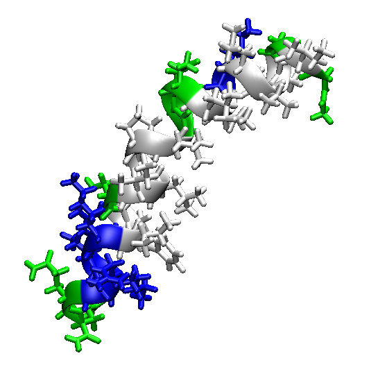
In this tutorial we will analyze a trajectory from an implicit solvent simulation of bee venom melittin. This particular
trajectory is from a single replica of a temperature replica exchange simulation. This means that the temperature
fluctuated during the simulation (between 300 and 400K) and non-native conformations may have been sampled that would normally
not be seen in a constant-temperature simulation at 300K.
We will use the MMTSB ensemble tools to post-process the conformations from the trajectory with clustering and an
MMGB/SA energy analysis to estimate the relative free energies at 300K of the sampled conformations.
|
|
1. Processing of trajectories
Download/copy the DCD trajectory file traj.dcd and the PDB file for the melittin
starting conformation melittin.pdb into your current working directory.
The DCD file is a binary file that may not be compatible with the computer you are working on. You can regnerate the DCD
file by downloading the complete tutorial package and running the script makeTrajectory.sh in the data
subdirectory.
We will now process the trajectory file to generate an ensemble data structure with the following command:
checkin.pl -dcd melittin.pdb traj.dcd -dir ens traj
The result is a new directory where each conformation from the trajectory is stored in its own subdirectory.
The name of the directory is given with -dir, it is ens in this example, and the conformations
are stored under the tag traj. The first conformation from the trajectory is stored as ens/0/1/traj.pdb,
the second as ens/0/2/traj.pdb, the 112th conformation as ens/1/12/traj.pdb and so on. Feel
free to explore the directories. You will notice that each PDB file is compressed automatically to preserve disk space.
The advantage of this type of data organization is that it is now easy to generate derived structures,
for example by minimizing each conformation. Having the data in this format is also a prerequisite for using the MMTSB
Tool Set ensemble analysis functions that are introduced in this tutorial.
2. Clustering
A common way to begin analyzing the conformations from a trajectory is through clustering based on mutual similarity
(according to RMSD). The following command will cluster the conformations in the ensemble:
enscluster.pl -dir ens -kclust -radius 2 traj
The Tool Set provides access to both K-means and hierarchical clustering algorithms. In this example, the K-means
algorithm is used (-kclust) with a radius of 2 Å. Other parameters in this command specify the directory
where the ensemble data is located and the name of the tag for the structures to be clustered. This tag should
match the tag that was given with the checkin.pl command above.
The results of the clustering can be retrieved with the following command:
showcluster.pl -dir ens traj
The output should look like this:
  t              212     3
    t.1             62     0
    t.2             45     0
    t.3            105     0
In this case there are 212 structures in total that fall into three clusters of comparable sizes. The clusters
are named t.1, t.2, and t.3 which will be needed in the next commands.
How do we find out which structures belong to each cluster? The command ensfiles.pl lists the files
in a given cluster as for example for the first cluster:
ensfiles.pl -cluster t.1 -dir ens traj
You should have seen a list of 62 files as a result of the following command. Now, which structure is most useful
to represent this cluster? The number in the last column gives the distance of each structure from the cluster center,
the most representative structure is typically the structure that is closest to the cluster center. We can find that
structure easily with the following command:
ensfiles.pl -cluster t.1 -dir ens traj | sort -k 2 -n | head -1
Find the representative structures for the three clusters and visualize them using VMD. Can you see what is
different between the different clusters?
Keep in mind that the structures in the ensemble are compressed and although ensfiles.pl shows
the file names without the ,gz extension you will need to use gunzip to unzip and copy
the files as in the following example before you can view the structures with VMD:
gunzip -c 0/1/traj.pdb.gz > struct.1.pdb
3. Analysis
We will now further analyze the conformations from the trajectory. In particular, we will carry out a quick
energetic analysis to determine the relative free energies of each of the three clusters at 300K that we found
above. Conformational free energies can be estimated with the MMGB/SA method by simply adding up the internal
vacuum energies of the solvent to implicit solvent free energies of solvation. For a single structure this is
accomplished with the following command:
enerCHARMM.pl -par gb melittin.pdb
In order to calculate the energies for each of the structures in the ensemble we use ensrun.pl which
can apply an arbitrary command to the ensemble of structure. This is called 'ensemble computing'.
ensrun.pl can take advantage of parallel computing facilities. In the following example we will
use two cores to accelerate the calculation of MMGB/SA energies:
ensrun.pl -cpus 2 -set deltag -dir ens traj enerCHARMM.pl -par gb
The resulting energies are stored under the name deltag. Once the command is finished the results can
be retrieved with:
getprop.pl -prop deltag -dir ens traj
The last command also takes the -cluster argument to limit the output to structures in a given
cluster:
getprop.pl -cluster t.1 -prop deltag -dir ens traj
In order to determine the relative energies between different clusters we need to average the free energies
for the set of conformations in each cluster. This could be accomplished with getprop.pl but it
is easier to use another tool, bestcluster.pl, which automatically calculates averages and ranks the
clusters accordingly:
bestcluster.pl -prop deltag -dir ens traj
The output from this command should look like this:
  t.3            105   105    -496.8737   37.4370    3.6535
  t.1             62    62    -492.1894   36.1223    4.5875
  t.2             45    45    -480.3959   44.2739    6.6000
For each cluster it shows the average energy (column 4), the standard deviation (column 5), and the
statistical error of the average based on the standard deviation and the number of samples (column 6).
In this example, the third cluster (t.3) has the lowest free energy, although the difference between the
average energies of the third (t.3) and first (t.1) cluster is not statistically significant
according to the errors. However, the structures in the second cluster (t.2) have significantly higher
energies.
Which structures have the lowest free energies in each cluster?
We can use ensfiles.pl again to find out which structures have the lowest free energies, this
time by using the -sort option with the deltag property name:
ensfiles.pl -sort deltag -cluster t.3 -dir ens traj | head -1
For convenience, this can also be done by adding the -lowest option
to bestcluster.pl as in the following command:
bestcluster.pl -prop deltag -dir ens -lowest traj
Finally, we will calculate the coordinate root mean square deviation of each structure in the ensemble
from the starting structure, again by using ensrun.pl:
ensrun.pl -set rms -dir ens traj rms.pl -fit -out CA `pwd`/melittin.pdb
This time we use rms.pl to carry out the RMSD calculation. The reference structure is given with
the full path (by substituting the current working directory with `pwd`) because ensrun.pl works
by going into each of the ensemble subdirectories before running the given command. If the absolute path
was not given, the reference structure melittin.pdb could not be found.
The resulting data is stored under the name rms and can be extracted again with getprop.pl.
Redirect the output from getprop.pl to a file and use gnuplot to plot the evolution of RMSD
as a function of simulation time. Frames in this trajectory are stored every 50 replica exchange cycles, where
each cycle consists of a 1 ps molecular dynamics simulation, so that the conformations in this trajectory
are spaced 50 ps apart.
We can now use bestcluster.pl again to find out how the average RMSD varies between the
different clusters:
bestcluster.pl -prop rms -dir ens traj
and more easily we can simply print out the RMSD of the best-scoring structures by
specifying the rms property with the -xlowest option:
bestcluster.pl -prop deltag -xlowest rms -dir ens traj
What do you find? Do the clusters with the two lowest energies have the lowest RMSD from the
initial (native-like) structure?
|