Objective and Overview
In this tutorial we will introduce the CHARMM polarizable force field based on the
fluctuating charge model of polarization. This force field is presently fully parameterized for proteins, water and a number of small molecules [1-3]. It can be utilized for simulations of proteins and peptides in water, as we will illustrate here by setting-up and running a short molecular dynamics simulaition of a mutant of the B1 domain of Streptotoccal protein G that forms a domain swapped dimer [4].
This protein as a monomer consists of N- and C-terminal β hairpins with a central α-helix. In forming the domain-swapped dimer, a hairpin from one of the protein chains exchanges with its neighbor. This is illustrated on the right.
To begin this tutorial you will need to download the files 1PGB.pdb and 1Q10.pdb from the PDB. Although we will not use the monomer structure, it is interesting to study it in conjunciton with the dimer and see how the exchange occurs.
|
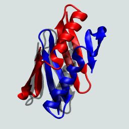
The GB1 domain-swapped dimer. Structures flash between the dimer and the monomeric GB1.
|
In this exercise, we will exploit the "bootstrapping" methods of combining use of the MMTSB Tools Set and CHARMM scripting to rapidly prepare our system. Because the MMTSB Tool Set has not yet been extended to accomodate the relatively new polarizable force field models, we will use the "standard" non-polarizable force fields in the initial preparation of our system and then switch to the polarizable force field when we begin simulations with CHARMM scripts.
|
- Patel, S & Brooks, CL, III. CHARMM fluctuating charge force field for proteins: I parameterization and application to bulk organic liquid simulations. J Comput Chem 25: 1-15 (2004).
- Patel, S, Mackerell, AD, Jr. & Brooks, CL, III. CHARMM fluctuating charge force field for proteins: II Protein/solvent properties from molecular dynamics simulations using a nonadditive electrostatic model. J Comput Chem 25: 1504-14 (2004).
- Patel, S & Brooks, CL, III. Fluctuating Charge Force Fields: Recent Developments and Applications From Small Molecules to Macromolecular Biological Systems. Mol Simul 32: 231-49 (2006).
- Byeon, IL, Louis, J, & Gronenborn, AM. A Protein Contortionist: Core Mutations of GB1 that Induce Dimerization and Domain Swapping. J Mol Biol 333: 141-152 (2003)
|
Extracting the protein structure
We must first extract one of the protein models from the pdb file 1Q10.pdb that
you just downloaded. This is an NMR structure and consequently contains about 50 separate NMR structures. We will do this using the MMTSB Tool
convpdb.pl. During
the course of extracting the peptide from the pdb file we want to (i) "convert" from generic pdb residue
naming convention to the "charmm22" convention for atoms and residues, (ii) center the protein, (iii) and create separate pdb files for the combined structure and each of the two chains in the dimer. The following commands accomplishe this:
convpdb.pl -center -model 1 -out charmm22 -segnames 1Q10.pdb > 1q10_a+b.pdb
convpdb.pl -center -chain A -out charmm22 1q10_a+b.pdb > 1q10_a.pdb
convpdb.pl -center -chain B -out charmm22 1q10_a+b.pdb > 1q10_b.pdb
Note that the output has been directed to the files 1q10_a+b.pdb, 1q10_a.pdb and 1q10_b.pdb
(you can download these files here if you are having troubles). Visualize the structure using vmd
to ensure you have what you want.
Now minimize the initial structure using the MMTSB Tool minCHARMM.pl to produce 1q10_a+b_min.pdb, which you can download here if needed.
Note that for these initial phases we are using the conventional CHARMM force
fields. We will switch to the polarizable force field below. The MMTSB Tools
do not have the full support for polarizablility yet, and thus we "cheat". The following command minimizes the peptide using a simple r-dielectric "solvent" model and the cmap extended force field. One thousand steps of steepest descents minimization is used with restraints (5 mass*kcal/mol/Å2) on the heavy atoms of the proteins. Each protein is terminally blocked with the ACE and CT3 blocking groups.
minCHARMM.pl -par minsteps=0,sdsteps=1000,sdstepsz=0.02 \
          -par trunc=switch,dielec=rdie,cutnb=12,cuton=8,cutoff=11 \
          -par param=22 \
          -par blocked,nter=ace,cter=ct3 \
          -cons heavy self 1:112_5 -log mmtsbmin.log \
          1q10_a+b.pdb > 1q10_a+b_min.pdb
|
Adding solvation
In this section of the tutorial, we will use the MMTSB Tools to solvate our minimized peptide. First we'll add solvent and then we'll minimize the complete system with harmonic restraints on the peptide. The system will then be ready for molecular dynamics runs. We do this all in two steps using convpdb.pl and minCHARMM.pl.
First use convpdb.pl to solvate and add segment names - extract the boxsize! We are using a truncated octahedral volume for this example. Note that this is really a minimal box ( 6 Å Cutoff ) for illustrative purposes, in general one would want at least 9 Å around the protein.
|
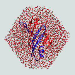
Does your solvated protein look like this? |
convpdb.pl -out charmm22 -solvate -octahedron -cutoff 6 1q10_a+b_min.pdb | \
           convpdb.pl -out charmm22 -segnames > 1q10_a+b_solvtmp.pdb
It is neccesary to assign separate segment names for the protein and water. However, this must be done in separate steps using convpdb.pl. We need to first extract them by using:
convpdb.pl -renumber 1 -setchain W -segnames -nsel water 1q10_a+b_solvtmp.pdb > 1q10_water.pdb
convpdb.pl -nsel protein 1q10_a+b_solvtmp.pdb > 1q10_protein.pdb
Now put them back together with
convpdb.pl -segnames -merge 1q10_water.pdb 1q10_protein.pdb > 1q10_a+b_solv.pdb
|
Now minimize with restraints and SHAKE constraints using PME electrostatics. Explore the minCHARMM.pl documentation a bit to understand the command below.
minCHARMM.pl -par minsteps=0,sdsteps=200,sdstepsz=0.02 \
	     -par trunc=switch,cutnb=12,cuton=8,cutoff=11 \
	     -par param=22 \
	     -par blocked,nter=ace,cter=ct3 \
	     -par shake,boxsize=58.413132,boxshape=octahedron,nblisttype=bycb \
	     -cons heavy self 1:112_5 \
	     -cmd mmtsbminsolvate.inp -log mmtsbminsolvate.log \
	     1q10_a+b_solv.pdb > 1q10_a+b_solvmin.pdb
We can further cheat and use the info garnered from our use of the MMTSB Tools above to build the CHARMM input script. We use the minCHARMM.pl -cmd command to build a CHARMM input file template containing the information necessary to build the psf in CHARMM. We utililze this file mmtsbminsolvate.inp to help build our polarizable force field CHARMM input file below. You can obtain an example of this file, here, but you will have to edit the PDB filenames accordingly.
|
Running molecular dynamics with the fluctuating charge force field
In this section we will take the configuration we just generated and run 0.5 ps of molecular dynamics on this system (1000 timesteps). This calculation takes about 15 minutes on 3.0 GHz iMac and is thus too big for an extensive run. However, it provides an example of what we can do with other proteins. We note that for the ChEq model we need to use 0.5 fs timestep to maintain the charge degrees of freedom near 0K, so they adiabatically follow the Born Oppenheimer surface. We will, as we did in the minimization command above, employ periodic boundary conditions with Particle Mesh Ewald (PME) to account for the long-range electrostatics. Also, we run 1000 steps of molecular dynamics at 298 K in a constant pressure (NPT) ensemble. The pressure is maintained via the CPT algorithm and the temperature via the Nosé temperature bath. We save the energy output, the trajectory file (coordinates of the system versus time, in a compact binary format) and the final configuration. The calculation is run using the CHARMM input script protein_cheq.inp displayed below. This script relies on the coordinates we just generated (1q10_a+b_solvmin.pdb), the topology and parameter files for the CHARMM Polarizable Force Field (top_allcheq06_prot_cmap.rtf and par_allcheq06_prot_cmap.prm), and the coordinates we generated in the first step above. Look through the input script and review the CHARMM documentation file cheq.doc before you run the calculation, familiarize yourself with the commands to turn on and off as well as manipulate the charge degrees of freedom.
You run the calculation (in background) with the CHARMM command (note be sure to check the values of the variables nwat, watseq, protbase and length, the first line below is a quick way to check the number of water molecules and modify nwat in the CHARMM command line):
grep "W00W" 1q10_a+b_solvmin.pdb | grep "OH2" | wc -l
$CHARMMEXEC nwat=2622 watseg=w00w protbase=pro length=58.413132 \
            < protein_cheq.inp > protein_cheq.out &
The input script protein_cheq.inp is:
*  Run and analyze dynamics of the protein G domain
*  swapped dimer in TIP4P water using the fluctuating charge
*  force field.
*

!***REQUIRED INPUT VARIBLES***!
!
if @?nwat eq 0     set nwat = 2623         !number of water molecules
if @?watseg eq 0   set watseg = w00w      !segid for water
if @?protbase eq 0 set protbase = pro      !base segment name for protein
if @?length eq 0   set length = 58.413132  !dimension of solvation box

if @?seed ne 0 goto gotseed
  system "date +%H%M%S | awk '{seed=$0*2+1;print "* Title"; print "*"; \
          print "set seed = "seed}' > seed.stream"
  stream seed.stream
  system "rm seed.stream"
label gotseed

! Read in the default CHEQ topology and parameter files
open unit 1 read form name top_allcheq06_prot_cmap.rtf
read rtf card unit 1
close unit 1

open unit 1 read form name par_allcheq06_prot_cmap.prm
read param card unit 1
close unit 1

! We use the MMTSB Tool Set to assist in a number of these
! steps. First we generate the separate chains using the commands:
!convpdb.pl -center -model 1 -out charmm22 -segnames 1Q10.pdb > 1q10_a+b.pdb
!convpdb.pl -center -chain A -out charmm22 1q10_a+b.pdb > 1q10_a.pdb
!convpdb.pl -center -chain B -out charmm22 1q10_a+b.pdb > 1q10_b.pdb
!
!
! Then we solvate the system and minimize it initially using
! a nonpolarizable force field. See the tutorial example at
! http://www.mmtsb.org/workshops/mmtsb-ctbp_2006/Tutorials
! for details.
!

open unit 1 read form name 1q10_a.pdb
read sequ pdb unit 1
generate gb1a first ace last ct3 setup
close unit 1

open unit 1 read form name 1q10_b.pdb
read sequ pdb unit 1
generate gb1b first ace last ct3 setup
close unit 1

! The system was solvated with @nwat water molecules
read sequ TIP4 @nwat !Solvate with TIP4FQ water model
generate wat  first none last none setup noangl nodihe

! set up tip4p bisector
lonepair bisector dist 0.15 angle 0.0 dihe 0.0 -
       sele atom wat * OM end -
       sele atom wat * OH2 end -
       sele atom wat * H1 end -
       sele atom wat * H2 end

rename segid @{protbase}a select segid gb1a end
rename segid @{protbase}b select segid gb1b end
rename segid @watseg select segid wat end
rename resname tip3 select segid @watseg end
!minimized solvated coordiantes
open unit 1 read form name 1q10_a+b_solvmin.pdb
read coor pdb unit 1 resid
close unit 1
rename segid gb1a select segid @{protbase}a end
rename segid gb1b select segid @{protbase}b end
rename segid wat select segid @watseg end
rename resname tip4 select segid wat end

! Add OM site using coor shake
coor shake

coor copy comp

! set the usual fluctuating charge parameters
!  Masses are from Rick, Stuart, and Berne paper.
cheq norm byres sele segid wat end
cheq norm byres sele .not. segid wat end
cheq tip4 sele segid wat end
cheq flex select .not. segid wat end
cheq qmas cgma 0.000069 tsta 0.01 sele segid wat end
cheq qmas cgma 0.000069 tsta 0.01 sele .not. segid wat end

set angle =  109.4712206344907

calc cutoff = @length / 2
let cutoff = mini  @cutoff   12

set cutim = @cutoff
Calc ctonnb = @cutoff - 3
Calc ctofnb = @cutoff - 2

!  Set-up crystal parameters
crystal defi octa @length @length @length -
    109.4712206344907 109.4712206344907 109.4712206344907
crystal build cutoff @cutoff Noper 0
imag byres xcen 0 ycen 0 zcen 0 select segid wat end
imag byseg xcen 0 ycen 0 zcen 0 select .not. segid wat end

! Set-up required non-bonded options
faster 1
update -
bycb inbfrq -1 imgfrq -1 nbscale 1.5 -
e14fac 0 nbxmod -5 -  ! These are required for CHEQ dynaamics
cdiel eps 1.0 cutnb @cutoff cutim @cutim ctofnb @ctofnb ctonnb @ctonnb vswi -
Ewald kappa 0.320 pmEwald order 4 fftx 64 ffty 64 fftz 64 !PM

! set this up so we could branch to analysis of we so choose
if @?analysis ne 0 goto analysis
label dodynam

shake bonh tol 1.0e-8 param mxit 2000

! minimize configuration w/o fluctuating charge
mini sd nstep 100 nprint 10

! With the scale commands below, we can calculate the shift in
! the charges from initial values to values that are "equilibrated"
! to the new environment.

! Turn cheq on and minimize again
cheq on

scalar charge store 1  ! charges before equilibraiton

! First just the charges
mini sd nstep 100 nprint 10 -
cheq cgmd 1 noco

! Now the whole configuration
mini sd nstep 500 nprint 10 -
cheq cgmd 1

scalar charge store 2

! Loop over protein atoms and write data in a file to plot
open unit 1 write form name 1q10_a+b_min_0.dat
set return = frommin
set unit = 1
goto getdipole
label frommin

! Put a copy of the charges into the wmain array
! and we can use these to color the atoms.
scalar wmain = charge
open unit 1 write form name 1q10_a+b_fqmin.pdb
write coor pdb unit 1

open unit 1 write form name 1q10_a+b_fqmin_no-om.pdb
write coor pdb unit 1 select .not. type om end

! set up the Nose-Hoover baths for the charges
! the calling procedure is identical to the NOSE
! call for applying the bath to nuclear degrees of freedom
!
!  the "NOSE" is replaced by "FQBA"
!!!
! Here we use one bath for the solvent and one for the peptide
!!!
FQBA 3                           ! set up '3' baths
CALL 1 sele segid wat end        ! select the atoms that will be coupled
                                 ! to bath 1
COEF 1  QREF  0.005  TREF 1.0    ! bath parameters (usual meaning)
CALL 2 sele segid gb1a end       ! select the atoms that will be coupled
                                 ! to bath 2
COEF 2  QREF  0.005  TREF 1.0    ! bath parameters (usual meaning)
CALL 3 sele segid gb1b end       ! select the atoms that will be coupled
                                 ! to bath 3
COEF 3  QREF  0.005  TREF 1.0    ! bath parameters (usual meaning)
END

open unit 10 write form name 1q10_a+b_fq_0.res
open unit 11 write unform name 1q10_a+b_fq_0.dcd
open unit 12 write form name 1q10_a+b_fq_0.kun

! Set-up the dynamcis run
dynamics cpt leap start timestep 0.00050 nstep 1000 nprint 100 iprfrq 100 -
   cheq cgmd 1 cgeq 1 fqint 1 -   ! Turn on CHEQ stuff for dynamics
   firstt 298.0 finalt 298.0  twindl -5.0 twindh 5.0 iseed @seed -
   ichecw 1 teminc 0.0 ihtfrq 0 ieqfrq 0 ilbfrq 0 -
   iasors 1 iasvel 1 iscvel 0 isvfrq 10 -
   iunwri 10 nsavc 100 nsavv 0 iunvel -1 -
   iunread -1 iuncrd 11 kunit 12 - !{* Nonbond options *}
   ntrfrq 2000 echeck 100000 -
   pconstant pmass 100.0 pref 1.0 pgamma 20.0 - !  Constant pressure
   Hoover tmass 50.0 refT 298.0


scalar wmain = charge
open unit 1 write form name 1q10_a+b_fq_dyn.pdb
write coor pdb unit 1

open unit 1 write form name 1q10_a+b_fq_dyn_no-om.pdb
write coor pdb unit 1 select .not. type om end

! Loop over protein atoms and write data in a file to plot
open unit 1 write form name 1q10_a+b_dyn_0.dat
set return = fromdyn
set unit = 1
goto getdipole
label fromdyn

stop

label analysis

! open the relevant files for simulation output
open unit 10 read unform name 1q10_a+b_fq_0.dcd
open unit 11 write form name 1q10_a+b_fq_0.ene

traj iread 10

traj query unit 10
set cnt =  1
set last = ?nfile
set skip = ?skip

! Use the access to system to create the desired drectory
system "mkdir pdb"
label readtrj

    traj read

    open unit 1 write form name pdb/1q10_a+b_fq_@cnt.pdb
    write coor pdb unit 1 select .not. type om end

    energy cheq cgmd 1

    calc step = @cnt * @skip
    write title unit 11
    * @step ?ENER
    *

    incr cnt by 1
if cnt le @last goto readtrj

close unit 10
close unit 11

stop

!###################Subroutine getdipole####################!
!!!!
!!!!
!!!!   This routine assumes the charges have been stored in
!!!!    scalar arrays 1 (old charges) and 2 (new charges)
!!!!   and the the dipole data will be written to unit.
!!!!   The routine returns to label return.
!!!!   The dipole moment for the backbone and side chains are
!!!!   computed for each residue and written to file unit.
!!!!
label getdipole

define co select type c .or. type o end
define nh select type ca .or. type ha .or. -
       type n .or. type hn end
define sidechain select .not. ( co .or. nh .or. segid wat ) end

set icnt = 1
label dodipole

      coor dipole select co .and. ires @icnt end
      set co = ?rdip
      scalar charge recall 1
      coor dipole select co .and. ires @icnt end
      set coo = ?rdip
      scalar charge recall 2

      coor dipole select nh .and. ires @icnt end
      set nh = ?rdip
      scalar charge recall 1
      coor dipole select nh .and. ires @icnt end
      set nho = ?rdip
      scalar charge recall 2

      coor dipole select sidechain .and. ires @icnt end
      set sc = ?rdip
      scalar charge recall 1
      coor dipole select sidechain .and. ires @icnt end
      set sco = ?rdip
      scalar charge recall 2
      write title unit 1
      * @icnt @co @coo @nh @nho @sc @sco
      *

      incr icnt by 1
if icnt le 112 goto dodipole
scalar charge recall 2

goto @return

stop
After running the dynamics (it should take about 15 minutes on a 3.0 Ghz iMac), visualize the final conformation with vmd. To view the molecular dynamics trajectories with vmd, you need to read create a set of pdb files (since vmd doesn't know about the binary dcd format when polarizable sites exist). You can do this with CHARMM and the "analysis" subroutine in the input script above with the commands.
$CHARMMEXEC analysis=true watseg=w00w < protein_cheq.inp > analysis.out &
and when it finishes:
vmd pdb/1q10_a+b_fq_[1-9].pdb pdb/1q10_a+b_fq_[1-9][0-9].pdb
|

|
In exploring this data, we see from the figure that the charges are significantly polarized from their gas phase values. The figure shows the dipole moment of the neutral C=O and H-N-Cα-H groups in the deal state and after the dynamics run. One clearly sees the polarization affected by the condensed phase environent.
The analysis you just ran also produced a file with the energy of each configuration, plot this energy. Finally, if you are adventurous, modify the CHARMM script above to analyze the average dipole moment for each of these groups across the trajectory. This can be done by "programming" in the CHARMM scripting language using the scalar commands.
|
|