1. Recentering/orienting and removing water from the trajectory

  orient.inp

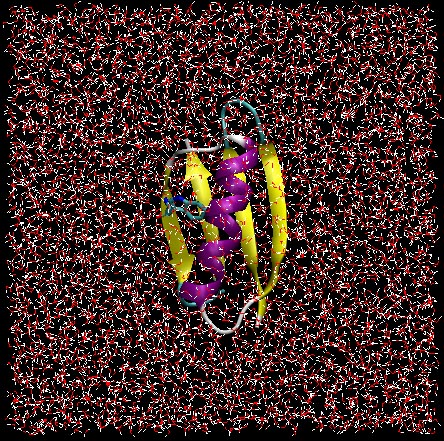
The raw trajectory often needs to be pre-process to facilitate some of the later analyses. The trajectrory was obtained from a simulation using periodic boundary conditions (PBC), which means that it is possible for the solute (the protein) to be partly out of the primary simulation box if we look at the raw trajectory. By recentering the trajectory we move solvent molecules, according to the PBC, so that the protein is in the center of the box in each frame. Furthermore we then re-orient each frame so that the protein is superimposed on the coordinates of the initial protein structure, thus removing overall protein rotation/translation motions. For a very flexible system the removal of overall rotation may be a non-trivial task, but grx1 is compact and quite rigid so we base the superposition on all atoms in the protein.

The script uses the CHARMM MERGE command (dynamc.doc) and demonstates only the part that we re-orient the protein and remove all water molecules. A new trajectory file is produced. The script also contains an example on how to re-center and orient the protein without deleting water molecules (this line is not excuted as it is after the "stop" command). MERGE can also be used to join or split trajectory files or to change (reduce) sampling frequency.

2. Root Mean Square Deviation and Radius of Gyration

  rmsd-singlepdb.inp  
  rmsd-rgyr-traj-correl.inp
  rmsd-rgyr-traj-corman.inp

Two simple characteristics of a structure are i) its RMSD wrt  to some reference structure (eg, the starting point of a simulation), which tells us something about the dissimilarity between the structures - 1 Å RMSD is barely visible to the eye, and RMSD 10 Å is very different, and ii) its RGYR, which is a combined measure of its overall size and shape. A sphere has the smallest RGYR of all bodies of the same volume increasing the volume, making the shape more anisotropic or having more of its mass at the periphery all lead to an increased RGYR. The proper definition of RGYR in mechanics is mass-weighted, which you can get by adding keyword MASS to the COOR RGYR command.

Three scripts are provided to demonstrated how one evaluate RMSD and RGYR using CHARMM. Script "rmsd-singlepdb.inp" is extremely simple and only calculates CA RMSD between two structures. Scripts "rmsd-rgyr-traj-correl.inp" and "rmsd-rgyr-traj-corman.inp" calculate RMSD and RGYR of a trajectory from a reference structure using two methods (CORREL vs. loop with CORMAN). In CORREL, the results could have been output to one file for each property, but we use the ability to edit the dimensions of the extracted time series in CORREL (edit ... veccod) to put all the information into one file.

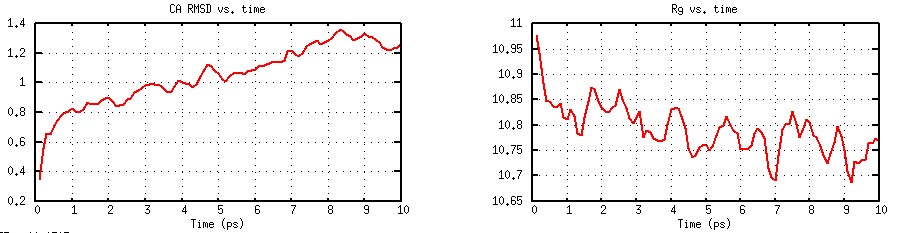
CA RMSD and Rg as functions of time (generated by "plot_rmsd.gnu").

3. Hydrogen Bond analysis

  hbond.inp

Hydrogen bonding patterns often provide useful information. In this exercise we use the COOR HBOND (corman.doc) command to find hydrogen bonds in a single structure, as well as average number of hydrogen bonds and their average life times from a trajectory. Hydrogen bonds can be defined in many ways, but we use a simple geometric criterion: A hydrogen bond exists if the distance between the hydrogen and acceptor atoms is less than 2.4 Å. This works well in practice. Note that when we have information about the hydrogen position, the hydrogen bond definition is not very sensitive to angular criteria, as are often used when determining hydrogen bonds in X-ray structures (lacking hydrogens). We will look at hydrogen bonds within the protein, between protein and water, and also on water-mediated hydrogen bonding contacts between different parts of the protein, ie hydrogen bonded interactions of the form A/D - water - A/D, where A/D denotes a hydrogen bond donor or acceptor in the protein. COOR HBOND uses the information about acceptors and donors in the PSF so we can use quite simple, and general atom-selections; all hydrogen bonds between the acceptors/donors in the two selections are calculated. A second form of the command (COOR CONTact) just applies the distance criterion to all the selected atoms.

The results are presented as hydrogen bonds per each acceptor/donor in the first atom-selection; if the VERBose keyword is present a break-down in terms of accptors/donors in the second atom-selection is given. NB! The VERBose keyword is not useful in a CHARMM loop when you want to extract total number of hydrogen bonds through CHARMM variables (subst.doc). <occupancy> is the average number of hydrogen bonds formed by a given accptor/donor during the trajectory.  The <lifetime> (in ps) is the average duration of each instance of a given hydrogen bond.

4. Secondary Structure

  2nd-structure.inp

5. Phi/Psi Distributions

  phi-psi-dist.inp

Peptide backbone dihdrals phi and psi determine the overall fold of a protein. In this example we extract histograms of phi and psi distribution from the trajectory for any selected residue using correl.doc. This script has the ability to take commandline arguments. The argument @rid has a default value of 41 by the virtue of the following command in the "phi-psi-dist.inp":

    if @?rid eq 0   set rid = 41

    $CHARMMEXEC rid=15 < phi-psi-dist.inp | tee phipsi.out

After the TRAJ command in the CORREL module has been executed averages and fluctuations are printed out for each time series. Both histograms are output to a single file named "phi-psi-dist.dat", and the phi/psi time series are output to "phipsi.dat". Following is a plot of of the results for Gly41.

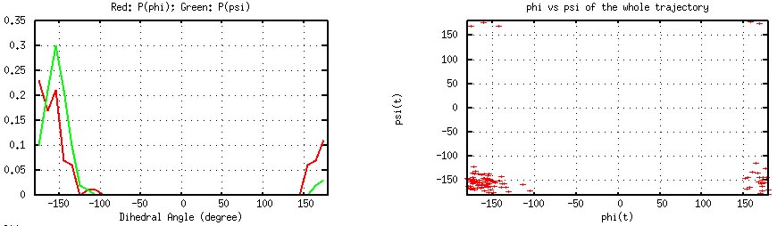
Gly41 phi/psi histograms (left) and time series (generated by "plot_phipsi.gnu").

6. Solvent Dynamics and Structure

  solvent.inp

All cells live an aqueous environment and their insides (cytoplasm) are also largely aqueous. Biomacromolecules thus have evolved to function with this in "mind" (membrane proteins are of course different in this respect); consquently CHARMM has well-developed facilities to analyze solvation behavior (see also the Hydrogen Bonds exercise). Here we will use the COOR ANAL (corman.doc) module to extract solvent dynamics (translational and rotational diffusion) and structure in terms of radial distribution functions. The example analyzes these properties for different regions of the water depending on the distance from protein surface (<5 A, 5-10 A, >10 A). As shown in the following plot, water molecules near the protein surface tend to diffuse and rotates slower (with larger effective rotational correation time and smaller diffusion constant). The Rg of different residues also indicate the degree of solvation.

Solvent structure and dynamics: MSD(t) (left), g(r) (center) and P2(t) (generated by "plot_solvent.gnu").

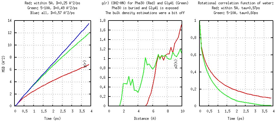
7. NMR Relaxation Rates and Generalized Order Parameters

  nmr.inp

MD simulations and NMR relaxation experiments often cover similar time-scales (ps-ns). Relaxation phenomena observed in NMR experiments depend on motional behavior of nuclear dipoles in the macromolecule, and the NMR module in CHARMM has been designed to allow efficient extraction of NMR related parameters from a trajectory (nmr.doc). This example analyzes relaxtaion parameters (relaxation rates, generalized order parameters, configurational entropy estimates) for the backbone amide groups.

Results, with some details such as the computed correlation functions are given in the output file "nmr-rt_ct.dat", and are also summarized in "nmr-r1r2.dat". Note that we use the trajectory with overall protein (translation)/rotation removed - we assume that internal and overall motions occur on very different time scales so that we can confidently separate these motions and focus on the internal motions. Such an assumption is necessary as most simulations are not long enough to sufficient sample global rotaional diffusion. The following figure plots the general order parameter S2 for each HN vector together with the secondary structure (generated by "2nd-structure.inp", see above). Clearly, even for a 10 ps simulation, it is evident that loops are more flexible (with smaller S2) (what a surprise. :D)

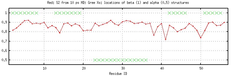
General order parameter and secondary structures (generated by "plot_nmr-s2.gnu").

8. Fluorescence Anisotropy

  trp--anisotropy.inp

The motion of chromophores may be detected by following the time-dependence of the polarized components of fluorescence emission following a brief pulse of polarized excitation. This time dependent anisotropy can also be computed from the (rank two) auto correlation of a unit vector along the transmission dipole (or, more strictly, the corelation between absorption and emission dipoles). Trp is the most useful intrinsic chromophore in proteins; Tyr also has a certain fluorescence, but less intense than that of Trp. Extrinsic probes (dansyl chloride and many others) are often used. The fast decay of this fluorescence anisotropy means that we usually can decouple the internal motions from the overall rotational diffusion of the protein (see also the nmr exercise). Protein G B1 only has one buried Trp. Within 10 ps simulation, Trp43 does not change rotamer state and the correlation fuction does not decay significantly.

Trp43 Ch1/Ch2 time series and dipole orientational correlation function (generated by "plot_trp.gnu").

9. Phi/Psi Based Clustering

  cluster.inp

As shown above in phi/psi distribution analysis, CORREL (correl.doc) can be used to extract time series of backbone dihedral angles (and many other properties). We can then use some of the dihdrals that vary during the simulation for clustering the structures in the trajectory. As shown from the rmsd analysis, the protein does not move much with 10 ps. We thus choose to use loop 38-41 that has the largest fluctation (or smallers order parameters from nmr analysis) to demonstrate clustering. The number of clusters and cluster centers are summarized in "clus-center.dat". Membership and distance from center of each frame are output in "clus-member.dat".